Reproducing Background Mortality
Rep_bgd_Canada.RmdIn this document, we aim to explore how the model behaves when COPD-related mortality is turned off. Specifically, our goal is to observe probability of death values that closely align with the background mortality rates from official Canadian sources. This is the expected behavior, as disabling exacerbation-related deaths causes the model to no longer predict mortality from exacerbations, which should result in values matching the background mortality rates.
To achieve this, we followed the series of steps below:
Step 1: Shutting off exacerbation related mortality.
First, we set the intercept of the exacerbation equation to a high value, effectively disabling death from exacerbations in the model. This adjustment is made by changing the relevant variable as follows:
library(epicUS)
packageVersion("epicUS")
#> [1] '0.33.99999'
input<-get_input()
input$values$exacerbation$logit_p_death_by_sex <- cbind(
  male = c(intercept = -13000, age = log(1.05), mild = 0, moderate = 0, severe = 7.4,
    very_severe = 8, n_hist_severe_exac = 0),
  female = c(intercept = -13000, age = log(1.05), mild = 0, moderate = 0, severe = 7.4,
    very_severe = 8, n_hist_severe_exac = 0)
)

#also setting exlicit mortality = 0 so there is no correction made
input$values$manual$explicit_mortality_by_age_sex <- cbind(
    male = c(rep(0, 111)),
    female = c(rep(0, 111)))
Step 2: Setting longevitiy-related parameters to 0.
Longevity is another factor in the model that influences population. To ensure that no external factors impact the population, we set these parameters to 0. This adjustment can be made in the input.R file.
Step 3: Run the model for 1 year and retrieve events matrix
Initially we run the model for 1 year and get the events matrix. This matrix logs all the events that individuals go through thoughout the model. We will use this matrix to calculate death probabilities produced by epicUS
library(epicUS)
settings <- get_default_settings()
settings$record_mode <- 2
settings$n_base_agents <- 3.5e5

init_session(settings = settings)
#> Initializing the session
#> [1] 0
# input <- get_input()

# set time horizon as 1 initially
time_horizon <- 1
input$values$global_parameters$time_horizon <- time_horizon

run(input = input$values)
#> [1] 0
events <- as.data.frame(Cget_all_events_matrix())
terminate_session()
#> Terminating the session
#> [1] 0

# checking to make sure event 7 (death by exacerbation) is not included
# because we shut that off in the model
unique(events$event)
#> [1]  0 14 13  5  6  3  4
table(events$event)
#>
#>      0      3      4      5      6     13     14
#> 350001   6726   1439  19794  19535   8699 350001
Step 4: Calculating probability of death from events matrix
library(dplyr)
library(tidyr)

# we will group by age so we convert ages into whole numbers.
events <- events %>%
  mutate(age_and_local = floor(local_time + age_at_creation))

# Filter events to identify individuals who have experienced event 14,
# while also creating a flag for whether they ever experienced event 13 (death)
events_filtered<- events %>%
  mutate(death= ifelse(event==13,1,0)) %>%
  group_by(id) %>%
  mutate(ever_death = sum(death)) %>%
  filter(event==14) %>%
  ungroup()


# calculationg probability of death
death_prob<- events_filtered %>%
  group_by(age_and_local, female) %>%
  summarise(
    total_count = n(),
    death_count = sum(ever_death==1),
    death_probability = death_count / total_count
  )
Inspecting the results
We should not consider 40 year-olds beause (Amin said … )
print(head(death_prob, 15))
#> # A tibble: 15 × 5
#> # Groups:   age_and_local [8]
#>    age_and_local female total_count death_count death_probability
#>            <dbl>  <dbl>       <int>       <int>             <dbl>
#>  1            40      0          16          16           1
#>  2            40      1           4           4           1
#>  3            41      0        4576           8           0.00175
#>  4            41      1        4607          13           0.00282
#>  5            42      0        4326          19           0.00439
#>  6            42      1        4519          16           0.00354
#>  7            43      0        4368          19           0.00435
#>  8            43      1        4496          13           0.00289
#>  9            44      0        4451          14           0.00315
#> 10            44      1        4476          10           0.00223
#> 11            45      0        4726          21           0.00444
#> 12            45      1        4756          15           0.00315
#> 13            46      0        4743          20           0.00422
#> 14            46      1        4743          11           0.00232
#> 15            47      0        4674          28           0.00599
print(tail(death_prob,15))
#> # A tibble: 15 × 5
#> # Groups:   age_and_local [8]
#>    age_and_local female total_count death_count death_probability
#>            <dbl>  <dbl>       <int>       <int>             <dbl>
#>  1            94      1         328          74             0.226
#>  2            95      0         265          81             0.306
#>  3            95      1         255          61             0.239
#>  4            96      0         197          71             0.360
#>  5            96      1         159          44             0.277
#>  6            97      0         115          40             0.348
#>  7            97      1          97          27             0.278
#>  8            98      0          85          32             0.376
#>  9            98      1          80          16             0.2
#> 10            99      0          59          31             0.525
#> 11            99      1          49          19             0.388
#> 12           100      0          51          29             0.569
#> 13           100      1          40          17             0.425
#> 14           101      0          43          12             0.279
#> 15           101      1          53          13             0.245
While these values are not perfectly aligned with our validation target, the variation is negligible.
Next, we want to ensure a consistent directional effect. We expect that increasing time_horizon to 5 years will bring the results closer to our target.
init_session(settings = settings)
#> Initializing the session
#> [1] 0

# set time horizon to 5
time_horizon <- 6
input$values$global_parameters$time_horizon <- time_horizon

run(input = input$values)
#> ERROR:ERR_EVENT_STACK_FULL
#> [1] -4
events5 <- as.data.frame(Cget_all_events_matrix())
terminate_session()
#> Terminating the session
#> [1] 0

table(events$event)
#>
#>      0      3      4      5      6     13     14
#> 350001   6726   1439  19794  19535   8699 350001

events5 <- events5 %>%
  mutate(age_and_local = floor(local_time + age_at_creation))


events5 <- events5 %>%
  mutate(local_time_adj = ceiling(events5$local_time))

# withing that year have they ever died?
events5_filtered<- events5 %>%
  mutate(death= ifelse(event==13,1,0)) %>%
  group_by(id,local_time_adj) %>%
  mutate(ever_death = sum(death)) %>%
  filter(event==14) %>%
  ungroup()


death_prob5<- events5_filtered %>%
  group_by(age_and_local, female, local_time_adj) %>%
  summarise(
    total_count = n(),
    death_count = sum(ever_death==1),
    death_probability = death_count / total_count
  )
#> `summarise()` has grouped output by 'age_and_local', 'female'. You can override
#> using the `.groups` argument.
Now, when we check the results. We see that the results are even further away:
print(head(death_prob5, 15))
#> # A tibble: 15 × 6
#> # Groups:   age_and_local, female [7]
#>    age_and_local female local_time_adj total_count death_count death_probability
#>            <dbl>  <dbl>          <dbl>       <int>       <int>             <dbl>
#>  1            40      0              1           5           5                 1
#>  2            40      1              1           4           4                 1
#>  3            41      0              1          16          16                 1
#>  4            41      0              2          12          12                 1
#>  5            41      1              1          10          10                 1
#>  6            41      1              2           6           6                 1
#>  7            42      0              1          20          20                 1
#>  8            42      0              2          14          14                 1
#>  9            42      0              3          13          13                 1
#> 10            42      1              1          10          10                 1
#> 11            42      1              2          10          10                 1
#> 12            42      1              3           6           6                 1
#> 13            43      0              1          12          12                 1
#> 14            43      0              2          17          17                 1
#> 15            43      0              3          14          14                 1
print(tail(death_prob5,15))
#> # A tibble: 15 × 6
#> # Groups:   age_and_local, female [7]
#>    age_and_local female local_time_adj total_count death_count death_probability
#>            <dbl>  <dbl>          <dbl>       <int>       <int>             <dbl>
#>  1           103      1              3           8           8             1
#>  2           103      1              4           1           1             1
#>  3           103      1              5           5           5             1
#>  4           103      1              6           6           1             0.167
#>  5           104      0              5           3           3             1
#>  6           104      0              6           3           2             0.667
#>  7           104      1              4           2           2             1
#>  8           104      1              5           2           2             1
#>  9           104      1              6           7           3             0.429
#> 10           105      0              5           1           1             1
#> 11           105      0              6           3           2             0.667
#> 12           105      1              5           1           1             1
#> 13           105      1              6           3           1             0.333
#> 14           106      0              6           1           0             0
#> 15           106      1              6           1           0             0
Visualizing results
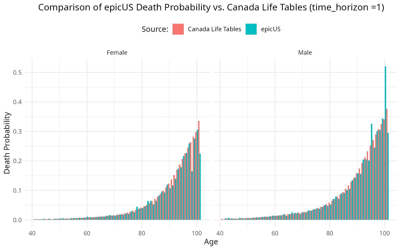
To better understand the differences, we visualize the results and compare them against the target values.
death_prob_clean <- death_prob %>%
   ungroup() %>%
   select(age_and_local, female, death_probability) %>%
   pivot_wider(names_from = female, values_from = death_probability, names_prefix = "sex_")

colnames(death_prob_clean) <- c("Age", "Male", "Female")
Canadalifetables_num <- input$values$agent$p_bgd_by_sex


Canadalifetables_df <- data.frame(
  Age = 1:nrow(Canadalifetables_num),  # Start age from 1
  Male = Canadalifetables_num[, 1],
  Female = Canadalifetables_num[, 2]
)

common_ages <- intersect(death_prob_clean$Age, Canadalifetables_df$Age)

# filter both so only include the rows with matching Age
death_prob_filtered <- death_prob_clean[death_prob_clean$Age %in% common_ages, ]
Canadalifetables_filtered <- Canadalifetables_df[Canadalifetables_df$Age %in% common_ages, ]
library(ggplot2)
library(dplyr)

combined_data_long <- bind_rows(
  death_prob_filtered %>% mutate(Source = "epicUS"),
  Canadalifetables_filtered %>% mutate(Source = "Canada Life Tables")
) %>%
  pivot_longer(cols = c("Male", "Female"), names_to = "Sex", values_to = "Death_Probability") %>%
  filter(Age > 40)

ggplot(combined_data_long, aes(x = Age, y = Death_Probability, fill = Source)) +
  geom_col(position = "dodge", width = 1) +
  facet_wrap(~Sex) +
  labs(
    title = "Comparison of epicUS Death Probability vs. Canada Life Tables (time_horizon =1)",
    x = "Age",
    y = "Death Probability",
    fill = "Source:"
  ) +
  theme_minimal()+
  theme(
    legend.position = "top",
    legend.justification = "center",
    plot.title = element_text(hjust = 0.5, margin = margin(b = 10))
  )
When time_horizon = 6, we get the following plot.
library(ggplot2)
library(tidyr)
library(dplyr)

combined_data_long5 <- bind_rows(
  death_prob5_filtered %>% mutate(Source = "epicUS"),
  Canadalifetables_filtered %>% mutate(Source = "Canada Life Tables")
) %>%
  pivot_longer(cols = c("Male", "Female"), names_to = "Sex", values_to = "Death_Probability") %>%
  filter(Age > 40)


final_EPIC_death5<- filter(combined_data_long5, Source == "epicUS")
final_Canada_death<- filter(combined_data_long5, Source == "Canada Life Tables")

# Add Death_Probability to Canadalifetables_filtered
Canadalifetables_filtered_long <- Canadalifetables_filtered %>%
  gather(key = "Sex", value = "Death_Probability", Male, Female)

# Loop through each unique year in the combined_data_long dataset
for (year in unique(combined_data_long5$Year)) {

  # Filter the data for the current year
  year_data <- combined_data_long5 %>% filter(Year == year)

  # Create the plot for the current year
  p <- ggplot(combined_data_long, aes(x = Age, y = Death_Probability, fill = Source)) +
  geom_col(position = "dodge", width = 1) +
  facet_wrap(~Sex) +
  labs(
    title = "Comparison of epicUS Death Probability vs. Canada Life Tables (time_horizon = 6)",
    x = "Age",
    y = "Death Probability",
    fill = "Source:"
  ) +
  theme_minimal()+
  theme(
    legend.position = "top",
    legend.justification = "center",
    plot.title = element_text(hjust = 0.5, margin = margin(b = 10))
  )

  # Print the plot for the current year
  # print(p)
}

print(p)
When we break it down and analyze per year, it seems to be in line with
what we expect.
When we break it down and analyze per year, it seems to be in line with
what we expect.
Eliminating smoking mortality
We have identified a potential source of the observed mortality discrepancies. Specifically, the mortality ratio associated with both former and current smokers appears to be influencing the results.
To investigate this, we set the following smoking-related mortality factors to 1 (indicating no excess mortality risk for former and current smokers):
After making this adjustment, the results align more closely with the life tables.
- This suggests that either:
- The model may be generating an excessive number of current and former smokers, leading to higher mortality than expected.
- We will need to update the mortality ratio estimates depending on whether an individual currently or formerly smokes.
input$values$smoking$mortality_factor_former<- c(age40to49=1,age50to59=1,
                                                 age60to69=1,age70to79=1,
                                                 age80p=1)
input$values$smoking$mortality_factor_current<- c(age40to49=1,age50to59=1,
                                                  age60to69=1,age70to79=1,
                                                  age80p=1)
#> Initializing the session
#> [1] 0
#> [1] 0
#> Terminating the session
#> [1] 0
#> `summarise()` has grouped output by 'age_and_local'. You can override using the
#> `.groups` argument.