Optimization
Optimization.RmdIn this vignette, we will walk through the process of optimizing
parameters for two equations: the longevity equation
l_inc_betas and the incidence equation
ln_h_bgd_betas. Specifically, we aim to optimize these
parameters to minimize the Root Mean Squared Error (RMSE) between the
projected population sizes and actual U.S. population data for certain
age groups.
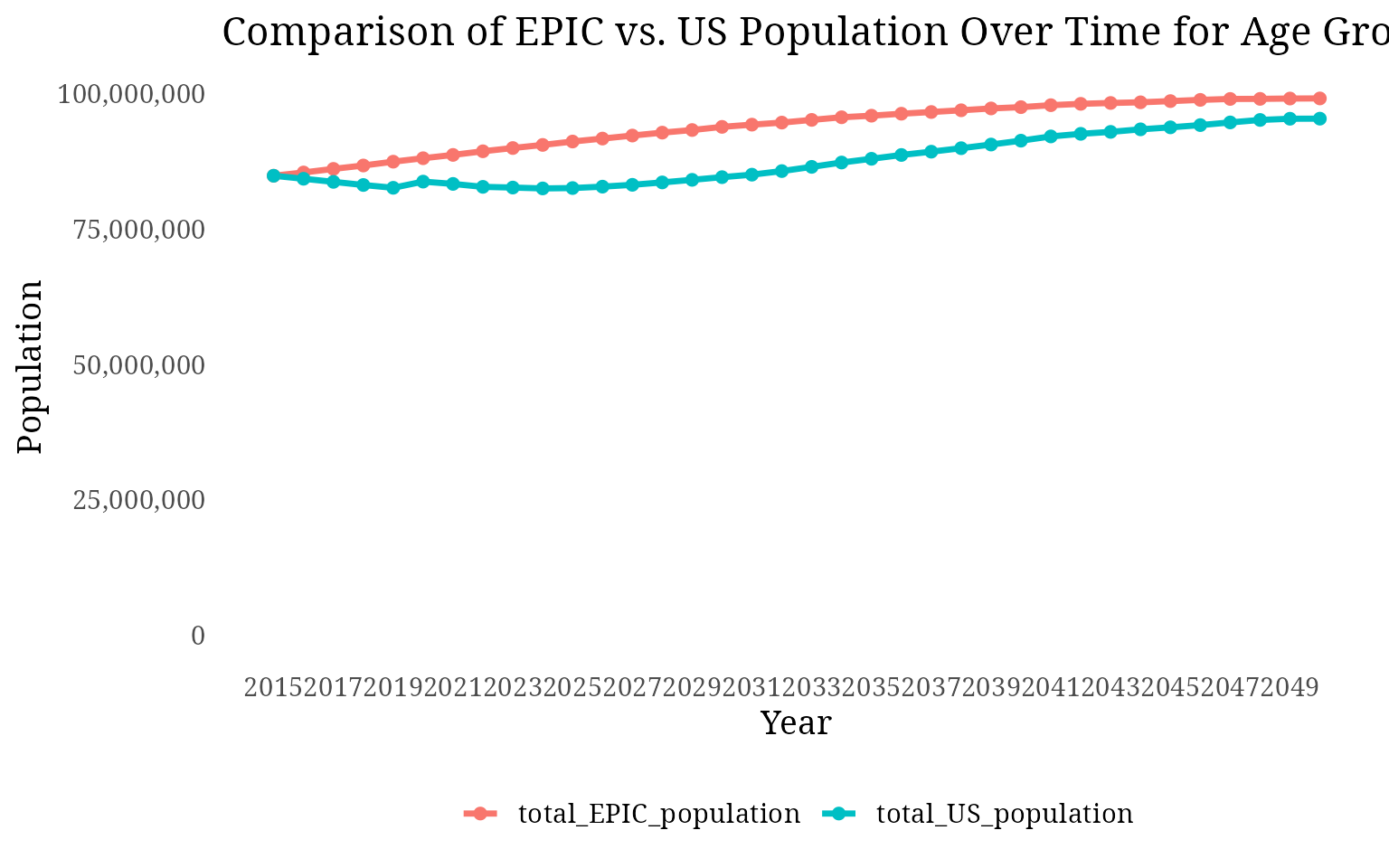
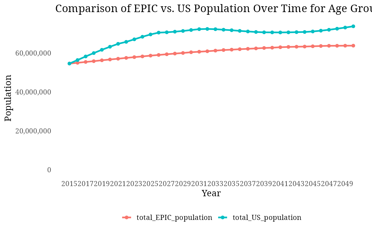
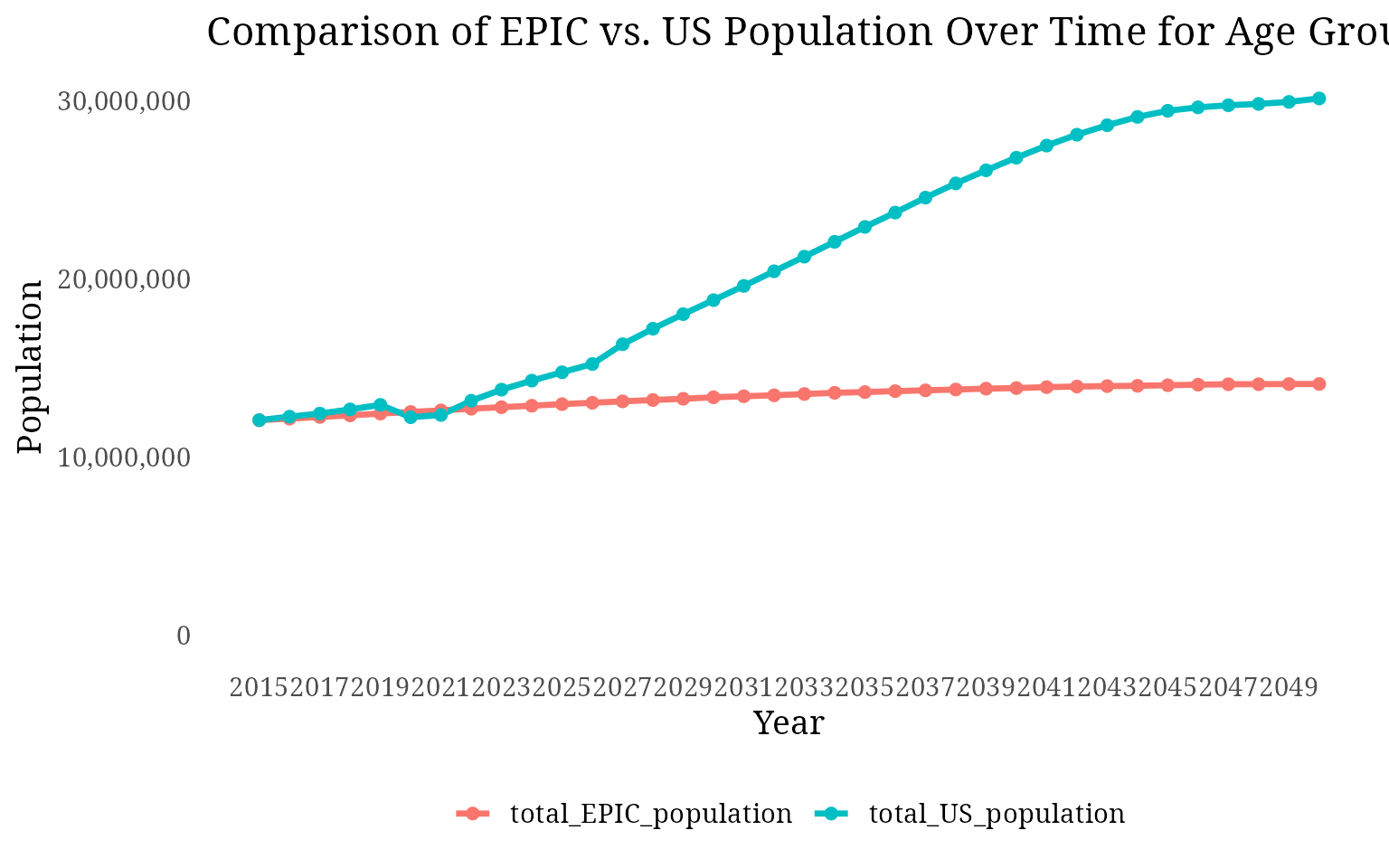
We perform optimization using the optim function in R, and the goal is to fine-tune the model’s parameters so that the RMSE is minimized. We focus on two specific age groups for optimization—40-59 and 60-79—while excluding the 80+ age group, as the RMSE for this group was significantly high, contributing excessively to the overall error.
Step 1:Load Libraries and Setup
Here, we load the necessary libraries. We also set the default simulation settings and specify the time horizon for the simulation (56 years).
library(epicUS)
library(tidyverse)

USSimulation <- read_csv(system.file("USSimulation.csv", package = "epicUS")

settings <- get_default_settings()
settings$record_mode <- 0
settings$n_base_agents <- settings$n_base_agents

input <- get_input()
time_horizon <- 56
input$values$global_parameters$time_horizon <- time_horizon
Step 2: Define the RMSE Calculation Function
The calculate_rmse_optim function calculates the RMSE
for each iteration of parameter optimization. Within this function:
- We assign the first three values of the parameter vector (params[1:3]) to l_inc_betas, which represents parameters for the longevity equation.
- The next four values (params[4:7]) are assigned to the ln_h_bgd_betas vector, which is part of the incidence equation. 3)The model is then run using the updated parameters, and we extract the projected population sizes (EPIC_popsize) and calculate the RMSE between the projected and observed U.S. population data for the specified age ranges.
# RMSE function for optimization
calculate_rmse_optim <- function(params) {


  init_session(settings = settings)

  #assigning first 3 values to l_inc_betas
  input$values$agent$l_inc_betas <- params[1:3]

  # assigning the next 4 values to the first four ln_h_bgd_betas, others = 0
  input$values$agent$ln_h_bgd_betas <- c(
    intercept = params[4],
    y = params[5],
    y2 = params[6],
    age = params[7],
    b_mi = 0,
    n_mi = 0,
    b_stroke = 0,
    n_stroke = 0,
    hf = 0
  )


  run(input=input$values)
  output <- Cget_output_ex()
  terminate_session()


  epic_popsize_age <- data.frame(year = seq(2015, by = 1, length.out = time_horizon),
                                 output$n_alive_by_ctime_age)
  colnames(epic_popsize_age)[2:ncol(epic_popsize_age)] <- 1:(ncol(epic_popsize_age) - 1)
  epic_popsize_age <- epic_popsize_age[, -(2:40)]
  epic_popsize_age_long <- epic_popsize_age %>%
    pivot_longer(!year, names_to = "age", values_to = "EPIC_popsize") %>%
    mutate(age=as.integer(age))


  validate_pop_size_scaled <- USSimulation %>%
    rename(US_popsize = value) %>%
    left_join(epic_popsize_age_long, by = c("year", "age")) %>%
    mutate(EPIC_output_scaled = ifelse(year == 2015, US_popsize, NA))

  # calculate total population and growth rates
  total_epic_by_year <- validate_pop_size_scaled %>%
    group_by(year) %>%
    summarise(total_EPIC_output = sum(EPIC_popsize, na.rm = TRUE)) %>%
    arrange(year) %>%
    mutate(growth_rate = total_EPIC_output / lag(total_EPIC_output))


  df_with_growth <- validate_pop_size_scaled %>%
    left_join(total_epic_by_year, by = "year") %>%
    arrange(year, age) %>%
    group_by(age) %>%
    mutate(
      EPIC_output_scaled = ifelse(year == 2015, US_popsize, NA),
      EPIC_output_scaled = replace_na(EPIC_output_scaled, first(US_popsize)) *
        cumprod(replace_na(growth_rate, 1))
    )

  # filter and sum population data by age group (40-59 and 60-79)
  df_summed_ranges <- df_with_growth %>%
    mutate(
      age_group = case_when(
        age >= 40 & age <= 59 ~ "40-59",
        age >= 60 & age <= 79 ~ "60-79"
      )
    ) %>%
    filter(age_group %in% c("40-59", "60-79")) %>%
    group_by(year, age_group) %>%
    summarise(total_EPIC_population = sum(EPIC_output_scaled, na.rm = TRUE),
              total_US_population = sum(US_popsize, na.rm = TRUE))

  # calculating RMSE of each age group across years
  rmse_per_range <- df_summed_ranges %>%
    group_by(age_group) %>%
    summarise(
      rmse = sqrt(mean((total_EPIC_population - total_US_population)^2, na.rm = TRUE)),
      .groups = "drop"
    )

  # summing all the age ranges
  total_rmse <- sum(rmse_per_range$rmse, na.rm = TRUE)

  print(paste("Params:", paste(params, collapse = ", ")))
  print(paste("RMSE:", total_rmse))

  return(total_rmse)
}
Step 3: Define Initial Guess, Bounds, and Run Optimization
We now define our initial guess for the parameters and set the bounds for each parameter. The optimization method used is L-BFGS-B, which is well-suited for differentiable functions with bounds. We also specify the stopping criterion.
initial_guess <- c(-3.5, 0.0005, -0.00005, 0, -0.025, 0, 0)

lower_bounds <- c(-3.6, 0.0001, -0.0001, -0.0005, -0.0001, -0.0005, -0.0005)
upper_bounds <- c(-3.45, 0.01, 0, 0, 0, 0, 0)


# here i am using L-BFGS-B because RMSE is a differentiable function
# we can define lower and upper bounds,
#more memory efficient in BFGS, making it suitable for large parameter spaces.
result_optim <- optim(
  par = initial_guess,
  fn = calculate_rmse_optim,
  lower = lower_bounds,
  upper = upper_bounds,
  method = "L-BFGS-B",
  control = list(maxit = 20, iterlim = 3)
)

print(paste("Optimal Growth Rate:", result_optim$par))
print(paste("Optimized RMSE:", result_optim$value))
Step 4: Optimal Parameters and Result
After running the optimization process, we obtain the optimal values for the parameters. These values minimize the RMSE for the specified age groups (40-59 and 60-79) and exclude the 80+ age group.
params <- c(-3.48672063032448, 0.00202274171887977, -4.37035899506131e-05,
            0, -1e-04, 0, -0.000132065698144107)
These are the optimized parameters that yield the lowest RMSE, and they reflect the best possible values for the model in terms of population size predictions for the selected age groups.